Notes on Synapses, Neurons, and Brains
On October 18, 2023, I started on the course Synapses, Neurons, and Brains with Professor Idan Segev. Below are my notes on the course. As always with notes, expect lots of abbreviated language and shortcuts. I also have some much more preliminary Review Notes.
Week One
Some dramatic billion-dollar projects include: * Allen Institute Seattle - Mouse/Human Brain Atlas * Janelia farm - DC, USA * EU Human brain project * President Obama’s “Brain Activity Map” initiative
Five exciting things:
Connectomix (see also Wikipedia article)
Brainbow
Brain-machine/Computer Interface (BMI)
Optogenetics
Computer Simulation of the Brain (e.g. Blue Brain Project)
Camillo Golgi and Santiago Ramon Y Cajal are “The Two Giants”, the beginning of modern neuroscience. Golgi stains actually only stain about < 1% of cells, so doesn’t make tissue dark, you can then see those stained neurons (a later term). 1906 Nobel Prize.
Connectomics
Connectomics is modern anatomy wiring diagram – cut very thin slices (nanometer resolutions). Electron microscope used for this. Detect slice structure separately, then reconnect slices. So it’s 3D mapping, so far done on pieces of brain, not whole brain.
Prospects for connectomics is to give us a complete blueprint of healthy and sick brain, and we may start to bridge the “structure-to-function” problem, and get into simulation-based research.
BrainBow
Genetic staining of neurons in vivo (light microscope – micrometer resolution). Harvard messing with mice genes, inserting pieces of DNA, when DNA is expressed, some cell types become colorful because of floursecent proteins (hence Brainbow). By the way, synapses are too small for this resolution, but can see general placement of neurons. Lot of art exhibitions based on this.
Prospects of this are 1) structural basis for learning; 2) taggging and genetic characterization of different cell types, eg. in retina, or find out how many cell types you have 3) Tracing connections in circuits, short and long range.
Brain Machine Interface
Electrodes implanted and listening to a single cell’s spike, or a large group of cells. Spikes are the common language. Talks to an Artificial Neural Network, and then to a robotic arm. Or can go the other way to ameliorate parkinsons, pulses from battery into basal ganglia. Basically a pacemaker for brain. Future challenges are 1) to be able to telemetrically record from within the brain without invasive electodes 2) real-time signal analysis. 3) Close the loop for movement with touching.
Optogenetics
Idea is to tweak the genetics of cells to plant probes that are sensitive to light, so you can shine light of particular wavelength and have it generate a signal. In nature, only retina is sensitive to light. But existence of retinal receptors means there are genes that can code for molecules that are sensitive to light. With two examples. Ion channel Rhodopsin spikes when blue light shines on it. C.f. Rhodopsin. Other example Natronomas pharaonis, yellow light prevents spikes. Movie from Janelia Farm (aka now Janelia Research Campus), can induce mice to drink with blue light on certain group of cells.
Blue Brain Project - Brain Simulation
Computer simulation (modeling) of neural circuits. Lord Kelvin (William Thompson) quote: “I am never content until I have constructed a mechanical model of the subject I am studying. If I succeed in making one, I understand; otherwise I do not.” [BL]
Uses powerful “Blue-Gene” IBM computer. Blue as in Big Blue, IBM. Modeling is writing equation to describe types of spikes for certain class of cells. Different equations for different spike (ultimately cell) types.
Modelling helps us to understand the network (e.g. by visualizing model in action).
So this is “simulation-based medicine [or s-b research]”
Week Two
The Neuron
The neuron
The axon
Dendrites / dendritic spines
Neuron types
Synapses
Electrical signals
Spike (action potentitial)
Post-Synaptic Potential (PSP)
Neuron as I/O Device
Historical perspective first, Hooke, Schwann, Golgi, Ramon Y Cajal, … and interestingly, Sigmund Freud (drawing crayfish neurons).
Nice images from Blue Brain, also videos of activity of living brain.
The Neuron Doctrine
Controversy between Camillo Golgi and Santiago Ramon y Cajal (RyC). Ramon y Cajal originally an artist. Looking through primitive microscope at different parts of nervous system in different animals, using Golgi staining method.
RyC by looking at anatomy only, conceived that information flows through axon, to and then to dendrites. Could not really see communication, drew arrows showing information flow, then thought from dendrite to cell body, to axon, to dendrite of next neuron. So theory that we’re dealing with individual cells is the neuron doctrine. The theory of dynamic polarization is that the receiving dendrite is somehow polarized, then flows to body, then axon.
N.B. RyC:
* Dendrites are the receptive devices (Input).
* Axons are the sending (output) devices.
We agree with this. Golgi did not like this – thought they were all connected physically. 1906 was a debate at the podium for Nobel prize.
Both axons and dendrites look like trees, axonal trees, dendritic trees. Axonal trees have varicosities (boutons) – this is where the neurotransmitters send the signal. Sometimes one axon will have 5,000 synapses
The neuron as an input / output device
NB: Really important introduction
NOTE: This video lesson has an excellent abstracted image associated with it.
Many (like up to thoushands) of axons (synapses) connect to one dendrite. Make little change in voltage, local synaptic potential. Certain types of cells (red in picture) make positive voltage (excitatory), the other ones are inhibitory. All together they sum the input, and the cell “decides” whether to generate an output yes or no. Output if there is one will be a set of spikes, tak tak tak etc.
Image too of pyramidal cell from cortex.
The Axon
Just after the soma, axon initial segment (AIS), hot region generating spikes. Consists of special ion channelss that make this region hot, i.e. enables generation of spike. This is where action potential starts, then it propagates down the axon, to all axon branches. Between axon segments are nodes of Ranvier. Between nodes of Ranvier are inter-nodes, with myelin sheath. Nodes of ranvier don’t have myelin sheath. Myelin is a lipid, it electrically isolates axon. Terminals of axon are pre-synaptic sites, boutons or varicosities; up to 5,000 per axon. No myelin on varicosity – it’s “bare wire”.
Myelin internodes generated by special set of non-neuronal cells. These are sometimes called glial cells, or have other names too that aren’t worth remembering but are oligodendrocytes. Electrical potential gets boosted in nodes of Ranvier.
Note that dendrites never have myelin.
By the way multiple sclerosis is a disease where the immune system attacks the myelen sheath, and messes with the signal flow.
Nodes of Ranvier amplify (boost) signal.
Summary:
Axon is highly branched structure emerging from soma. Can branch locally or go centimeters or even meters away from soma.
Starts with hot axon initial segment, where spike starts, then it propagates along axon.
Covered with myelin, except in nodes of ranvier, where there are hot ion channels
Has frequent swellings (boutons), where the neurotransmitter “hides” (pre-synaptic site).
Most importantly, axon is an output electrical device. It generates and carries electrical signals called spikes.
The Dendrite
10/20/2023
Pictures of dendrites (links below to 3rd party resources)
Purkinje cells from cerebellum, “small brain”. Flat, bush-like.
Starburst amacrine retina cells.
Pyramidal cell – common in hippocampus; pyramidal structure (triangular looking) cell body.
Point here is name of cell often depends on structure of dendritic tree.
RyC drawing shown pyramidal cell, with small branches, dendtritic spines, so this type is a spiney dendritic tree, and these spines are “where synapses are made onto”. Pyramidal cells are spiney. Sometimes 10,000 spines per pyramidal cell. On his death bed RyC was drawing spines.
Typical number for pyradimal cell in cortex:
total area 20,000 square micrometer [(= micron). One millionth of a meter]
each spine has area of 1 square micrometer of dendritic spines per cell, 8,000, average. But could be 30,000 or more.
Listen to 10,000 synapses
In cortex, in terms of area, 50-60% of brain area is dendrites.
Pictures of human pyramidal cells from cortex. Showing apical tree (point of pyramid) and basal tree (again see Pyramidal cell).
Takeaway: cortical pyramidal cells have dendritic spines.
Neuron Types
Can classify by:
Anatomical features (e.g. “face” of dendrites and axons)
Functional, .e.g. excitatory (principle) vs inhibitory (interneurons) – balance between two is very important, by way.
By electrical spiking pattern. Some cells fire more or less, different patterns.
By chemical characteristics.
Using gene expression
Count of neurons in human brain: a number close to 100 billion.
Work on this is not final. # of types not final, depends on classification, but could say several thousand types overall.
Example (detail on point 2), in neocortex, principle (excitatory cells) have long axon that projects to other brain regions, whereas interneurons (inhibitory) have local axonal projection.
2013 work by Javier DeFelipe to classify inhibitory neurons, Chandelier, large baskent, horse-tail, Cajal-Retzius, etc. etc. Depends largely in differences in dendritic tree or sometimes axonal structure. Why different structures an interesting question. [I also wonder if this needs to be modeled for an artificial (ANN) human.]
Slide of electrically-based (spiking) classification. Some fire a lot (regular). Some “stutter”. We don’t understand the structual reason for this.
The Synapse
The synapses is a chemical / electrical device that connects axon of neuron A to dendrites of nueron B. Pictures of very close axon - denrite connections. Single pre-synaptic cell can make contact at several locations to the same post-synaptic cell. Using electron microscope, can see axon bouton (pre-synaptic) connecting to dendritic spine (post-synaptic). They don’t physically touch, but very very small gap.
Side note when axon connecting to spiny dendrite, this is typically excitatory type connection. Electron microscope view showing showing axon A with small vesicles, a very small gap, and a dentridic spine, B – vesicles contain neurotransmitter, e.g. 5,000 molecules of glutamate, acytlcoline, or seratonin. So vessicles live in axonal varicosities (boutons). Neurotransmitter travels through gap to dendrite spine. Spike is digital, all or none. When spike arrives, secretes the neurotransmitter – spike is the trigger. Post-synaptic, you’ll also see a signal too, “excitatory synaptic potential”. So two types of activity:
Action potential (from axon)
Post-synaptic potential (could be excitatory or inhibitory)
Major difference is action potential is digital signal. The post-synaptic potential is graded, analog signal [this reminds me of how ANNs are modeled?]. So digital signal on one side to analog on other side. So digital-to-analog converter.
Slide on synapse vesicle quantal release.
The Neuron as Output Device: Part 2
Summary of Lesson 2
Different cell types.
Excitatory input can come from very far away, e.g., thalamus to the cortex.
Cell may receive 1500 synapses from neighbors, 360 from thalamus, etc.
Now reshow important diagram
In the receiving cells, have Excitatory post-synaptic potentials (EPSPs) and Inhibitory post-synaptic potentials (IPSPs) – eventually all gets summed up in the cell body, may reach threshold for action potential generation.
First quiz first attempt got 92.85% on attempt one, 10/21/2024
Week Three - Electrifying Brains – Passive Electrical SIgnals
The Cell as an RC Circuit
Today starting with passive properties. Already mentioned, pre-synaptic we have action potential, digital, all or none. In this lesson we’re talking about next part, the synatpic potential, in the dendrite. So in week 3:
link anatomical structure to idea of passive-RC circuit.
talk about membrane, and the membrane time-constant (Tau-M)
Temporal summation of repeated inputs – “electrical memory”
Generation of post-synaptic-potential (PSP) in post-synaptic membrande
Continue talking about excitatory (E) and inhibitory (I) synapses.
E & I interaction
Start with a small patch of membrane, can wrap it into a sphere. We’ll place an electrode, and record dif between inside and outside of cell (voltage). If we inject a positive current into cell, I (current), if you do this you see a voltrage change (V), the voltage change doesn’t look square like current we injected, but it grows over time as a smooth curve, also slowly drops when current stopped. So cell is not a mere resistor, because if it were, and you injected I, you would get a voltage that consists of I x R. (Ohm’s law - V = IR). Not like that, it takes time t to grow, and also to decay. We call curved response to I, we get a depolarizing current, i.e. becoming less negative.
When people saw this, they though that a cell that acts like an R-C circuit. If you inject I into such a circuit, it takes time to grow, and when stop injecting current, takes time to go back to baseline or zero. So RC circuit is a good approximation of such behavior.
The voltage equation for the passive cell
The math for an RC circuit, want to again measure V (voltage) in response to current (I):
Total current is either resistance current or capacitance current.
So capacitative current + resistance current is equal to Current (I).
This is basicall Kirchoff’s Law
If you solve this equation for V you get behavior of cell, solution is linear because C is constant, resistance is constant, current input (I) is constant. end up with dv/dt as a solution, which is a derviative, so shows change over time.
Initial conditions, V (t = 0) = 0, and up with some V after certain time.
At t = 0, e to zero is one, 1-1 = 0, so V(t = 0) = 0, or
If inject current for infinite time, e to power of -t goes to zero, so IR * (1 - 0) = IR so
This last is steady state.
So these are two ends.
The Membrane Time Constant
This time we want to look at \( t = RC \).
By the way, RC is many times called tau,
or sometimes
i.e. tau membrane.
Looking at t = RC = Tau, what is value of V. Well ends up being
So
The one minus e to the -1 is = .63, so
Can use same equation to ask how will voltage decay (attenuation) when we stop the current. So still exponential, but not 1 - exponent, just exponent. Attenuation like build-up.
Tau-M is caled the membrane time constant (very important).
Attenuation function is
Growth and decay are mirror images of one another, goverened by Tau-M, the membrane time constant. It governs how fast the voltage develops / attenuates. If time constant long, will take a long time to attenuate, and vice versa. (earlier I believe he said RC (tau) in seconds).
This constant in effect tells you about the electrical memory of cell. Short means it “forgets” quickly.
Another important parameter is R, sometimes called
R input, or input resistance.
R directly tells you maximum voltage you can reach for a given I. RC tells you how fast go up and down.
So critical parameters for passive RC circuits are:
R
RC
Temporal Summation
An important consequence of time constant, what if inject an intermittent current, not a constant one. So I is intermittent. Voltage goes up and then attenuates, but not all the way down, so following second period of I, get a buildup on top of remainder of previous one. This is called temporal summation.
If would have done it constantly, would have gotten a larger buildup. IR is maximum you can get.
Next shows negative current, here voltage will be pushed down. The name for this [mentioned in passing] is hyperpolarization. (When cell gets more positive, it’s called depolarization, or hypopolarization).
This temporal summation of positive and negative current is “exactly what synapses are doing”.
The Resting Potential
Now back to cell membrane (circle) near R/C diagram – this is the “Passive Membrane Model”.
New: When you implant the electrode into the cell, suddenly see a drop in voltage. I.e., cell is more negative than outside, so drop in voltage is from zero to “something like -70 mV” (millivolts).
So inside of cell is about 70 mV more negative than the outside of the cell. This is called the resting potential, i.e., with no current. This negative charge inside requires energy to maintain. In any brain, inside is more negative, so because of this we need to add a battery to the original RC circuit. (This appears to be a good related article).
Resting potential symbol:
Again: More positive: Depolarization More negative: Hyperpolarization
Next stage is to speak about synapses, which can add this current….
The Synaptic Potential, Part I
Up until now we’ve dealt with passive proprerties of cell, resting potential.
BTW, ballpark values for R * C, Time constant, = Tau, of on the order of 20 milliseconds
Brief review of synapse, vessicles of axon meeting receptors of dendrite – what happens when neurotransmitter interacts with receptors. We get new ion channels opened in the receptor, which enable the flow of current, either from out -> in or from in -> out. So on the dendrite side eventually, result of neurotransmitter uptake is new ion channels. Channel behaves like a conductor or a resistor, we call it
Wait – now talking about it as a battery for the synapse:
The Synaptic Conductance
Looking at dendritic side membrane, earlier said two types of channels.
One type is passive type that, in total, represent the R value (resistance) in the cell. (“white channels” for purposes of drawing)
Other type (“red channels” for purposes of drawing), when synapse interacting w/ neurotransmitter. These then are synaptic channels.
We represent the conductance of these with
for the r (resting channel), passive resistance, and
for the synaptic channels.
Red channels only open in response to reaction with a neurtransmitter. Collectively they result in something called the synaptic voltage.
But we need to also discuss the Synaptic Battery (next)
The Synaptic Battery
Difference in ion concentration is a general property of living cells. In particular in nerve cells. For instance, outside nerve cells there are a LOT of (positive +) sodium channels, and much fewer inside cells. In case of potassium, opposite is true, lots inside, less outside.
If you open a particular sodium channel only, because of concentration gradient, you will get positive flow into the cell. So will get depolarization, John says – and professor says a second later. :)
So calling it a battery is a way of representing the flow of ions.
For potassium, because there is more inside, it will flow from inside -> outside, so you will lose positive charge, so cell will become hyperpolarized.
The Synaptic Potential, Part II
So, again:
Post-synaptic membrane has both passive channel and synaptic channel.
Specific ion channels get opened, allows current to flow either in or out.
Circuit has \( g_{\space r} \) (g-rest), resting conductance plus resting battery, \( E_{\space r} \), the whole -70 millivolts – this is the passive part of circuit.
Synaptic part is \( g_{\space s} \) synaptic conductance plus \( E_{\space s} \), synaptic battery.
Equation before was \( C \frac{dV}{dt} + g_{r} (V - E_{r})\) First part is capacitative current, second part of that is passive current.
Now equation with red current (synaptic part):
\( C \frac{dV}{dt} + g_{r} (V - E_{r}) + g_{s} ( V - E_{s}) = 0 \)
Last term is synaptic current. Sum of all terms in above equation = 0 according to kirchoff’s law. You can solve this equation to get that last V – the voltage generated by the synapse.
The Voltage Equation for the Synapse and EPSP and IPSP
Again, the current equation is:
\( C \frac{dV}{dt} + g_{r} (V - E_{r}) + g_{s} ( V - E_{s}) = 0 \)
If solve it for V – the voltage change due to activity of synapse, you get this equation:
There is a ceiling to positive or negative synaptic battery.
Reasonable range is something like +200 millivolts to -90 millivolts. Whole world represented by signals in this range. :) If voltage goes up, it’s EPSP (Excitatory Post-Synaptic Potential). If it goes down, it’s IPSP (Inhibitory Post-Synaptic Potential)
Summary
EPSP and IPSP diagram, we have time consant – if both at both time, have temporal summation.
Quiz for this one done on 10/25/2023, got this nice little encouragement along with a 90% grade:

Week Four: Electrifying Brains - Active Electrical Spikes
The Hodgkin Huxley Experiments
Now talking about active signals – the spike! The all or none, digital phenomenon that comes from the axon. This again is the action potential (axon) – as opposed to resulting synaptic potential in the dendrite.
Outline:
The excitable (“spiking” axon)
The Hodgkin & Huxley experiments (Two giants)
Space clamp and voltage clamp
Membrane conductances/currents underlying the spike
Hodgkin & Huxley model for spike initiation (math. model)
Spike propogation along axon
From synapses to spikes
Two giants: Sir Alan Lloyd Hodgkin and Sir Andrew Fielding Huxley – both working in Cambridge before WWII. Nobel prize 1963. They used the squid as an experimental animal. Squid has unique property – a giant axon, that’s about 0.5 mm (500 micrometer) wide. (Axons in brain on the order of micrometers – too small to work on) This allows you to place an electrode (the long way, like a catheter). Published first view of spike (on oscilloscope) in 1939, by electrically signalling the cell. Needs stimulus strong enough in depolarizing direction. Starts from resting potential. Goes up, then goes back down below resting potential (but gradually creeps back up). Spike is about 1 millisecond long.
This is a universal activity of nerve cells.
Wrote beautiful set of 4 equations in several papers (1952). Now we understand action potential in a very compact way. “I see it as a triumph of theory. Actually I don’t think that today we have such a beautiful theory in neuroscience as the Hodgkin/Huxley theory for the spike.”
Membrane Currents Underlying the Spike
Example of a votage clamp – now changing voltage (Hodgkin and Huxley) by a fixed amount. So there is a voltage change. Behaves like a passive RC current – nothing new – if depolarizing current is sub-threshold. If depolarize further, “For suprathreshold depolarizing voltage clamp, the recorded membrane current (after the first capacitative current) flows first inwards (into the axon) and later outward (from inside to outside).” – this is a surprise. First see capacitative current as before – as you hold voltage – see first an inward current into the axon, then curves up. Remember, voltage is fixed, but then get inward then outward current.
Found that if you used drug, tetrodotoxin (TTX), a fish toxin, if put it on axon, the inward phase disappears, left only with the outward phase. With tetraethilammonium (TEA) – now the outward current gets blocked, but leaves inward. What they found by playing with Na and K concentrations, that inward was Na and outward was K.
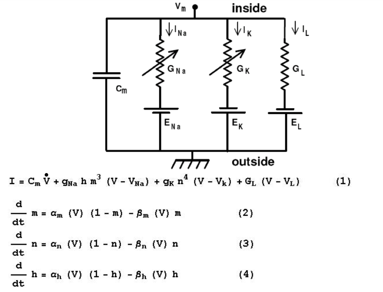
Found sodium current was inward current (fast – happens early on) – then changes to potassium current later (outward current). Outward current continues if continue voltage clamp. In 1954D paper by Hodgkin / Huxley, circuit diagram of squid axon.
Have Capacitive current + Early sodium current + later potasium current + leak current (resting state cell is negative).
Modeling the Membrane Currents
I.e. for first one, membrane voltage minus the potassium ion battery times the conductance = the current. Same for sodium. In voltage clamp case, we fix \( V_{m} \). Can try different values of \( V_{m} \)m, measuring conductance of potassium and sodium. Important: Degree of conductance depends on voltage. Get more conductance of both depending on voltage.
Summary:
The slow (K) current (conductance) does not inactivate during voltage clamp (VC)(outward).
The K conductance rises slower than it decays at the end of VC.
The fast (early) Na conductance inactivates during VC.
H. & H. fitted an equation. The fact that it grows slower and attenuates faster, rising phase described as function $\( (1 - exp(-t))^{4} \)\( and the decay as \)\( exp \space (-4t) \)$
So then they wrote this equation: $\( \newcommand{\overbar}[1]{\mkern 1.5mu\overline{\mkern-1.5mu#1\mkern-1.5mu}\mkern 1.5mu} \)\( \)\( g_{K} = \overbar{g_{K}}^{n^{4}} \)$
Right hand side, “g-k-bar”, is maximum conductance, but actual conductance depends on term n – which is the voltage. When it’s zero, no potassium conductance. When n = 1, you get maximum conductance since \( 1^{4} = 1\) Can also say n repesents the proportion of K-ion channels in the open state. Tried to relate that 4 to the number of ions are in a certain region of the membrane.
The H&H Spike Model
Talking about potassium channel. Can think about \( n^{4} \) as having four gates. Need to move all 4. Say zero means it’s closed. Can think about n as a probablity, because in range 0-1. So probablity must be n = 1 to get to all of them to open.
Already saw activation function:
The rate function that \( n \) depends on in turn is
Basically this says you move from open state to closed state as a function of both voltage and time. \( \alpha \), if big, shifts close state to open state, and \( \beta \) shifts shifts open state to closed state. \( \alpha \), becomes larger with voltage \( \beta \) becomes smaller with voltage.
Sodium equation a bit more complicated.
First means that \( m \) opens the channel very fast, but \( h \) closes the channel more slowly. Two differential equations that follow show how m and h change with time. Because now dealing with \( m^{3} \), sodium channel has (schematically) three gates. m gate opens early but h gate closes the channel but slowly.
Now can see that this prediction and math by H&H, now know that there are parts of channels that are voltage sensors, m fast and starts it, h slower and turns it off.
When you solve equations for V, which appears in quite a few places, you can graph the spike that you actually see. Since values are voltage dependent, e.g. for sodium, as voltage increases, this opens up channel even more.
Variable notes (mine):
\( m \) - Sodium activating variable
\( h \) - Sodium de-activating variable
\( n \) - Potassium activating variable
At same time that start with de-activation of sodium with h variable, also get activation of potassium with the n variable. So it’s an extra help to hyperpolarization. (Hence overshoots below baseline).
The Refratory period:
You can’t get a second action potential very early after first one – have to wait enough time. It’s about 10 milliseconds for full action potential. So maximally, 100 spikes per second. This is an experimental finding. H&H explained it with behavior of both \( h \) (inactivation) variable and the potasium conductance. Both h and K conductance are slow.
Can see spikes in any nerve cell, e.g. squid (as we’ve discussed), or cortical pyramidal cell.
In living cell, this is a result of cell being de-polarized enough by voltage received from synapses of up 10,000 dendrites (if not too many inhibitory cells).
Note: This one was the toughest quiz so far and the only one yet that I’ve had to re-do.
Week Five - Neurons as Plastic/Dynamic Devices
Outline and Introduction
Fast examples
Purpose of learning (“action perception loop”)
Functional plasticity (learning w/o anatomical changes)
Structural plasticity (where anatomy does change)
Discussion on memory: Embedding memories. Copy memories? Is it reliable?
New thing 2013 Nature Karl Deisseroth et al published, “The Clarity Method”. Idea to develop methods to make whole brain transparent. c.f. Bringing Clarity to Brain Research video. Remove coating of brain and stain different cells different colors, make it transparent and “fly around” in it.
Aristotle quote on memory – not groundbreaking. :)
What changes in brain when you learn.
Some ambiguous or not clear images shown – teach you how to interpret them.
Amir Amedi - Hebrew University – Sensory substitution for the blind. Can we use sound?
Learning [looks like this slide is on Machine Learning] enables us to:
Generate useful predictions.
Categorize the world (“faces”, “cars”, etc.)
Create consensus among us for successful interaction.
Movement essential for perceptual learning (“action-perception” loop) - active cat vs. passive cat. (Held & Hein experiment).
Mechanisms Subserving Learning and Memory
The brain reconstructs reality from minute/very partial information (e.g. cochlear implants). In this case, get strange noises in your ear, but you can interpret it. Brain has to reconstruct it.
Also true of vision, for example.
Now, brain mechanisms supporting functional and structural plasticity. How does what we’ve learned feed into this.
We start again with Santiago Ramon Y Cajal. Believed that nerve cells do not multiply [not correct], so he believed that learning resulted in more dendritic processes and axonal “colllaterals” – so important point is more connections. Thought cerebral cortex like “a garden filled with trees, the pyramidial cells, … multiply their branches …”
Hippocampus very very important for learning and memory. Looks like a sea-horse [sort of], hence, hippocampus. But not only this – also study the cortex.
Possible neuronal mechanisms underlying learning & memory:
New nerve cells grow - new functional neural networks relate to new items (structural plasticity). Cajal didn’t know aobut this.
New synaptic connections (structural plasticity). Ramon Y Cajal believed this.
Strength of existing (synaptic) connections change, becoming stronger or weaker – functional plasticity. (Donald Hebb)
Functional Plasticity
The Hebb Hypothesis: (Donald Hebb 1949 – likely here) “When an axon of cell A is near enough to excite cell B or repeatedly or consistently takes part in firing it, some growth or metabolic change takes place in one or both cells such that A’s efficiency, as one of the cells firing B, is increased”
aka “Fire together/wire together”
Subsequent investigation has shown that Hebb’s rule is indeed implemented at some (hippocampal and cortical) synapses. So synapse is highly plastic device. So after learning, for example, for same spike (axonal) get stronger EPSP (Excitatory post-synaptic potential) in dendrite of cell B – more depolarization. E.g. insertion of additional receptors to post-synaptic membrane. More ion-channels post-synaptically. Could also do pre-synaptically, same spike could release more transmitters.
Now we can add electrodes to both cells and try to figure out mechanism. Doing this led mainly in 1990s to Spike Timing-Dependent Synaptic Plasticity (STDP). If generate with electode pre-synaptic (A cell) spike and post-synaptic (B-cell) spike, enough times, then you get a larger EPSP as in last paragraph. Depends on timing between pre-synaptic and post-synaptic spike. We call result, Long-Term Potentiation (LTP) – for hours, days, lifetime.
If reverse order of timing (B then A) then you can make the connection weaker. Called LTD – Long Term Depression. See this in Slide based on Dan and Poo work in rat visual cortex, 2006, curve trending downward. Trends upward if A then B. Also shows smooth curve based on time (timing dependent). For times > +/- 40ms, no effect. Incidentally, this doesn’t explain the Pavlov case since bell/food could be seconds away.
We can write the equation for LTP/LTD. Really blurry slide.
Structural Plasticity
“Morphological/anatomical changes that are correlated with learning”
Here talking about dendritic spines, it seems.
1967 - Globus & Scheibel [one of many experiments]. If cover eyes (visual deprivation) of an animal (cat? rabbit?), you see changes in the density of the spines.
In response to learning, see increase in number of stable new “spines”.
Until recently, all of this was learned on dead brains, before and after learning or deprivation. Now we have the 2-photon microscope to view spines in living brain tissues. Can see changes in real-time in living brain in response to learning, see changes in dendritic spines.
“Spines appear and disappear frequently in the adult cortex.” Some are stable, but others appear and disappear. So morphological changes and new synaptic connections all the time – but does it relate to plasticity? Yes!
Also strength of the synapses increases. As it becomes stronger, it persists longer. So…
New dendritic spines are born constantly.
More during learning tasks/enriched environment.
New spines associated with new synapses – i.e. new functional networks.
Neurogenesis and Learning
Are there new-born cells (neurogenesis) in the adult Brain?
Yes, in song-birds, in adult males, when they sing new song. Controversial until recently in mammals. Pasko Ravic thought only new cells in prenatal and early postnatal. But in 1997, Elizabeth Gould at Princeton showed neurogenesis in tree shrews, and in 1997 in marmoset monkeys (primates :)). At least two regions where this happens: olfactory system and hippocampus.
In mouse, more challenging task (learn to wait to respond to a tone), the more newborn cells you develop. These are born from stem cells in hippocampus, some of them are integrated in network. Questions are what makes them stable or not.
Neurogenesis provides hope for Alzheimer’s and Parkinsons, as well as rehab from stroke / brain injury.
“If you don’t use it, you lose it.” Challenge is good.
Comments and anecdotes about memory:
Hippocampus of London Taxi Drivers
Whole brain structural differences between musicians and non-musicians (increasing volume – could be from spines, or cells)
Future - controversial issues
Machine learning
How trustworthy are memories?
Can we read out memories? (Generally, no, because you code things differently from other people)
Can we stimulate brain to embed new memories. Difficult to know how to manipulate network correctly.
Week Six: Cable Theory and Dendritic Computations
The Brain Computes
Focus of this week is on computation, especially computational capbabilities of dendrites.
“The brain computes (thus ‘computational neuroscience’).”
Computation at level of single neurons
Focus on very important, fundamental “cable theory for Dendrites” (William Rall)
Dendritic computation - the neurons as a computing device.
Recent experimental breakthroughs that prove the these ideas of neurons as computing devices, e.g. the retina.
Start with this “The Brain Computes” – how do neuronal ingredients (neurons, synapses, electrical and chemical signals, their networks etc.) “represent and process information (compute)”?
What are the problems that need to be solved by the brain?
What are the algorithms (techniques) to solve the problem?
How do [are] these algorithms implememented by the various brain regions.
Each region has a computational role - slide showing this. E.g. movement (crossing street, reaching for cup), compute distance of objects like cars, movement, speed, direction. Movement and vision together. In visual system other things to compute. E.g. figure/ground, recognizing objects in world. Brain has a particular algorithm to compute faces, e.g. classical example with just faces and pixels showing where your eyes focus. Shows an algorithm for finding the face, not a full scan of whole image. Another one in profile.
Other figure ground – four pac-man figures oriented the right way make a square.
Also motion – visual system sensitive to motion.
Computation at the level of Single Neuron
Computation is “main mission of brain”. Single cell already shows aspects of computation – most direct example, from Nobel Laureates Hubel and Wiesel, 1981 Nobel. Recording spiking activity of cat visual cortex during visual motion. Recording electrode in living, seeing cat. So particular cell was firing in a paticular occasion – whenever there was a line crossing the screen at a particular angle. Recorded from V1, part of the visual area (primary visual cortext), from a single cell. If line crossing screen at a different angle, does not fire. So cell is orientation/direction specific cell. A given cell will fire more strongly or not fire at all for these: _ | / \ etc. One he showed fired strongly for vertical, a bit for just off of vertical, other orientation not at all. So cell is tuned for particular range of angles, strongest at center of range.
V1 is early in visual system, we decompose the world into lines.
Fundamentals of Dendritic Cable Theory
Before this, early theoretical ideas about neuron as computational device – influential early paper was McCulloch and Pitts “point neuron”. “A logical calculus of the ideas immanent in nervous activity” (1943) – was influential in computer science as well. Ideas inspired by:
“all or none” nature of the spike
Two types of synapses, Excitatory (E) and Inhibitory (I)
Abstract (point) neuron, has all or none property – it fires or doesn’t. [He’s basically going to end up with boolean possibilities I bet. – YEP! :)] Assumes single cell I can veto, and three excitatory cells, can write:
“Output (“1”) is generated if: (e1 OR e2 OR e3) AND NOT i. Again this is a logical calculus. So now neuron is logical device, with thresholds. Showed that with these simple properties, can build a universal computing machine, using connected networks of such neurons. By the way a lot of the mathematics for computers was influenced by neurons. So “basically the first example of looking at neurons as computing devices.”
But neurons (dendrites) and their syapses are not “points”, but distributed electrical systems So what are the computational implications? For this need a conceptual framework and rigorous theoretical approach.
Goes back to the importance of mathematics – Lord Kelvin I think he misquotes him?
“I am never content until I have constructed a mechanical model of what I am studying. If I succeed in making one, I understand; otherwise I do not.”
Professor has “mathematical” in there.
Thompson did like his math, though, e.g.
“When you can measure what you are speaking about, and express it in numbers, you know something about it, when you cannot express it in numbers, your knowledge is of a meager and unsatisfactory kind; it may be the beginning of knowledge, but you have scarely, in your thoughts advanced to the stage of science.”
Why Model (in Details?)
Three reasons for mathematical models:
Correct interpretation of experimental results (provides experimental predictions!). Go from details to predictions.
Gain insights into key biophysical parameters (enables compact description of the physiologicaql behavior studied capturing the essence, e.g. HH model for the AP). So allows you to zero in on key parameters, important features.
Enables you to jump conceptually from biophysics to computation, i.e. functional. E.g. M&P neuron – and next thing we’ll talk about, Rall’s ideas for dendritic computation (next slide).
But first a bit about our friend Ramon y Cajal – he didn’t like theoreticians. Bunch of anti-theorist quotes from “Advice for a young scientist”
Rall Cable Theory for Dendrites
Wilfrid Rall was “my [Professor Idan Segev’s] own great mentor”.
Goal here is to understand the impact of (remote) dendritic synapses (input) on the soma/axon (output) region. Rall [Wikipedia: “one of the founders of computational neuroscience”]. Wrote paper in 1964 showing contrast between M&P point neuron (AKA schematic neuron) vs real neuron. The real neuron distributed, much more complex. Thought M&P was too oversimplified.
First intuition came about in 1959 – if inject current into cell (soma) or current comes from synapses, can see, most of current flows through out to dendrites and not into the soma membrane, so can’t think of soma as isopotential because of all the dendrites popping out.
Dendrites are not isopotential devices, but a distributed electrical system. Therefore:
Voltage attenuates from synapse to soma
It takes time delay for the PSP to reach soma
Somatic EPSP/IPSP is expected to change with synaptic location
So Rall showed it schematically as dendritic tree as sets of cylinders. A distributed system, again. Asked, what does it mean for electrical behavior.
Now look at cable theory:
Suppose you have cylinder, has a membrane, and inside dendrite, and inside there are chemicals etc. that act as a resistance (hence, more or less, acts like a cable). Suppose you activate it at some location of the cylinder. Ion channel flows into (for example) across membrane. Some flows left and right in cylinder, and a bit leaks out of the cylinder (dendrite) too. So membrane voltage attenuates as you go away from synapse, maximum voltage is local. So question is how to describe the attenuation of of voltage across a branching tree structure mathematically.
In brief (simplifying the math somewhat). Idea is basically you have an axial current that is proportional to the derivative of voltage with distance. ( \( \frac{\delta V}{\delta x} \)). Change in actual current actually second derivative.
Much longer passive cable equation given. Change in current is basically sum of cable current and membrane current. Passive current because r and c (resistance and capacitance) are static (passive). So current changes with both distance and time.
Linear partial differential equations that can be solved analytically, if you have initial conditions and boundary conditions – dimensions of cylinder and voltage. Rall solved it for various initial conditions. Can assume steady state (no change in time), voltage still attenuates with distance, shape of attenuation depends on properties of cable (infinite vs a sealed end cable so no current can escape, etc.). For short branch, almost no attenuation.
Most fundamental and important solution of cable equation was for branch dendritic tree model – in this case steep (assymetrical) voltage attenuation from dendritic synapse to soma. Steep attenuation of voltage to first branch site, more shallow as we go closer to “trunk” of three. At boundary of cable, have a leaky end, hence steep attenuation. Eventually some voltage reaches soma. So this is very non-isopotential system, high voltage near synapse, low at soma. Maybe 30 or 40 millivolts at synapse, but only see one millivolt at the soma.
Another thing that falls out is get less attenuation at soma if inject current directly there.
Now think about dendrites as “functional subunits” or “synaptic territory”. If synapse near cell body, soma and cell body about the same. Each synapse has a neighborhood, or sub-region; distal part less affected. We can use notion of regional sub-units as doing computation.
Transient synapses
Relationship not only to X (distance), but also T (time) – so with time, voltage dissipates distally as well. If wait enough time, cell becomes more isopotential, resting synapse.
Distal synapses have a broader curve (not so much local voltage initially). “Distal synapses are broader and delayed” was a predictive result of cable theory, compared to proximal synapses. If normalize peaks just to compare shape, distal synapse is delayed and broader. Can plot time to peak, then plot half-width. So can use shape curve of EPSP, can predict how far away the synapse is that caused the EPSP. This a big success of theory – later experimentally verified.
Now take Rall mathematics and look at the cell as a computational element…
Dendritic Computation
A few theoretical ideas that came out from Rall’s (better :) Cable theory.
Dendrites enable neurons to act as multiple functional subunits. So dendrites may be computing locally first, then globally at the soma and axon.
Dendrites because distributed can classify inputs.
Important - neurons with dendrites can compute direction of motion (directionally selective)
Dendrites improve sound localization (in auditory system)
Dendrites can sharpen the tuning of cortical neurons
First back to neurons as as multiple functional subunits. Distributed multiple functional subunits ideas means (Koch and Poggio) can extend (write more precise but complex) version of the logical calculus of M&P. If closer (proximal), inhibition can veto. So inhibition / excitation. All inibitory synapses “on the path” (proximally to soma) can veto you. – “on the path” conditions.
Another idea (Bartlett Mel) is notion of functional sub-regions performing preliminary summation (non-linear operations), and then sum the local operatrions. So clustering of synapses in sub-regions can affect output differently than if didn’t have it. B. Mel showed that this allows neuron to act as a classifier. E.g. image of face gets projected to different regions of a cell. So one cell may be sensitive to a given face. So individual cell becomes a classifier.
Most influential original idea is Rall, 1964, is that neuron can behave as directional selective computation device. Moving from proximal to distal codes one direction, reverse codes reverse. Temporal order switches. EPSP at soma will have a different voltage profile. More distal first will have a taller voltage curve because will sum up with proximal, but spike will happen later. Smaller peak but broader if proximal first. Could have a threshold between the two to make output depend on which direction. Spike in one case and not the other. Say you have a directional selective cell in retina. Can distribute photoreceptors along the cable. With Rall’s cable theory, then, built up directional cell (a computation). Can’t do this with a point neuron.
Rall suggested that you have to be careful about the “granularity of the model” needed to explain the phenomenon. So, for example, point neuron can’t compute directional sensitivity on its own, as we saw above. So Rall suggested going up only so far as you need to understand a particular computational phenomenon. Rodin’s detailed model of a kiss as example, vs. Brancusi’s simplified kiss… . Overly detailed model more like a simulation.
Recent Breakthroughs
“tour de force” as attempt to understand neurons as a computing device. For example, direction of motion. Two experimental breakthrough.
Arthur Konnerth in Munich. Nature paper 2010. Using two-photon microscope. Mouse watching lines move in one direction or other – electrode recording of different direction. Spikes in two directions – one much stronger than other. If you zoom into input synapse. Different synapses “like” different directions. So we’re in a “miraculous time” - not only record output of cell (summation of inputs), but also record from input synapse itself. All orientations are presented to various synapses, but each synapse sensitive to particular orientation. We don’t know yet how it creates output corresponding to orientation. Could be that cell counts the orientation of majority – or another mechanism.
Second result is direction sensitivity in retina ganglion cells. How is it computed?
Retina built up in layers (in order distal to proximal)
Receptor layer - neurons that receive the light.
Bipolar cells
Amacrine cells
Then to ganglion cells (optic nerve) [Optic nerve “is composed of retinal ganglion cell axons and glial cells” - wikipedia]. SOME of Ganglion cells are directionally senstive – spikes for certain directions of motion. Tuned cells. Before cortex [ before Hubel and Wiesel].
HOW?
One idea over the years was the “Reihard Detector” – general idea is that in one direction there is more inhibition, than in other direction. So assymetry of location of E & I connections into ganglion cells. Depends on whether E or I happens first for a given direction. If I comes in after E – too late. Just an idea, but how do you prove / disprove it?
Answer: Connectomix - Kevan Martin, Winfrid Denk, and others, cutting and reconstructing anatomy and electrophysiology at level of synapses. Recently breakthroughs – from Winfid Denk and his team, shows indeed, if look at DS Ganglion cell, and it’s predecessor, the Amacrine (inhibitory) cell, can count the inhibitory synapses. If have three cells for example:
Amacrine 1 -> DS <–Amacrine 2
If one have more synapses, can count the synapses. E.g., if more on 2, get more inhibition to the right, for example. [amacrine cells are all or primarily inhibitory]. So this could be a verification of Reihard detector idea.
Personal note
Brain differs from other large physical systems in which elementary units are simple and uniform. “It is composed of neurons which are inherently complex, dynamic, and plastic units, which form connected networks that exploit the impact of the individual neuron.
Analogy to indiv. humans and society.
Need conceptual and theoretical tools for connecting low level computation and learning to global computational functions. This the central role of new field of “computational neuroscience.”
Only tight integration between theory / modeling will provide missing breakthrough.
Week 7 Cortical Networks - Out of the Blue Project
Cortical networks - out of the blue project.
Mega projects for the brain. Blue Brain part of several.
The cortex and its “cortical column”
A test-case for large-scale details modeling (the blue brain project)
The Human Brain Project
Some dramatic new ($ billions) projects for the brain
Allen Institute Seattle - Mouse/Human Brain Atlas - mouse/human brain atlas, and now gene expression of brain related genes. Recent focus on visual system.
Janelia farm - DC, USA - Work on connecting network level anatomy and pysiology to a specific behavior. Somewhat futuristic. Very new.
EU Human brain project - Professor is involved. Lausanne, Switzerland. New platforms for research, integrates knowledge from different disciplines.
President Obama’s “Brain Activity Map” initiative - “Brain Activity Map”. Creating revolutionary tools to measure/simulate of millions or even billions of neurons simultaneously. Record many spikes in living brain. Hope to see what happens in coding, decoding, etc.
The “diseaseome” - the 560 known neurological diseases.
Attempt to systematically link genes to certain diseases, and other correlations. Part of big attempt worldwide – also part of Human Brain Project. All a result of misbehaving anatomy or behavior (e.g. spiking behavior) or both. Hagai Bergman’s work on Parkinsons – showing different activity of brain region vs. Parkinson.
The Blue Brain Project
Before the Human Brain Project. Idea was:
Build new platform for databasing the brain. (I added, see GitHub Repo). This part not controversial. Controversial part is simmulation. Data enables visualization and reverse engineering via simulation. Platforms for collecting and preserving data. Platform at all levels, from genes to behavior.
Generate simulated spikes and so on, of neurons. This controversial. Whole field is called simulation-based researched, simulate in fine detail the system you study. Question is – is that reasonable, useful, etc.
Like reverse engineering, rebuilding a simulated brain – hoping you’ll understand via simulation. Henry Markram started BB project – later head of human brain project. IBM provided the “Blue-Gene” supercomputer (earlier used to sequence human genome) 10,000 processors, 0.05 Peta Flops / sec. So blue comes from IBM. [hints at a sexual connotation too.] Data-basing the brain was assisted major new anatomical methods:
BrainBow. (Design mouse genetically so that cells intrinsically will have color.) Other anatomical tools too. Now can see certain types of cells standing out.
Connectomics – also controversial – Labor intensive, EM slices. Cells “reconstructed” in computer and colored. Controversy is about – OK, so now you have all this data what do you do with it?
Other technique related to BAM, in vivo optical recording of electrical activity of thousands of neurons – use Ca-sensitive florescent dyes + 2-photon microscope. Can now see individual cells of a living mouse, for example, and study it while it’s doing specific tasks.
The Cortical Column
So we choose a circuit and reconstruct it so we can simulate it. What should we choose? The cortical column. If look at mamalian neurocortex, and look at skull side and go two mm deep, see layers and layers of cells. Ballpark, \(1\space mm^2 \approx 30,000\) cells, 100 million connections (synapses). Cortex has many cell types: “Some of the cells are pyramidal cells, we discussed them. Some of the cells are spiny stellar cells. Some are inter-neurons. Some are inhibitory. Some are excitatory. Many, many cell types within, a circuit like this.” There are layers in the cortical columns – layer means cell bodies of certain cells is denser there. Or may be some layers less dense than others. (Slide showing layers approx 2 mm x .46 mm). Slide of spiny stellate cells in cat v1 in layer 4, attempt to map out all the input synapses into cell (yellow coming from the thalamus, green are regional). So statistical synaptic mapping of the local cell region. (Kevan Martin et al).
Location of synapses, firing sequences, I vs. E, etc. all part of what we enter into our simulation.
The Cortical Column Network
Now move from individual cells to networks of cells. Slide of the mouse whisker and the barrel cortex. This system well defined anatomically. Somato-sensory cortex, different columns for each indiv. whisker. Each column on order of 10,000-20,000 cells. Diagram showing cortex column surfaces seems to be aligned corresponding to layout of whiskers, notion of column an active area of research – clear mapping between whisker and a column. E.g. Bert Sakmann, noble laureat. Slide showing excitatory cell types, e.g. pyramidal layer 5 cells, spiny stellate cells in layer 4, etc. Typically six layers, other showing input from thalamus. Can also stain cells, exitatory red, inhibitory green, etc. – map types into a column.
Some other functional properties of columns:
Orientation of moving lines. Mentioned this in Hubel and Wiesel - Clay Reed discovered that in the cat V1, we have a whole functional column that is sensitive to a particular direction. Columns tend to go in order, with orientaion changing a bit between each one. If look at different axis from surface, other axis is oriented according to left eye / right eye. This is called the “ice cube model” of visual cortex.
The functional unit (the column) is plastic, not just indiv. cells. For example, can show cat limited visual angles in world at early age, and only those respective columns formed in V1.
Blue Brain Project
Modeling the cortical column
We need to model all that stuff we mentioned before about connectivity, cell types, firing properies, etc. – but we don’t understand how these ingredients generate a response. For that we need to model it.
Blue Brain Simulations
We have not only anatomy of many layers, but each cell has its own properties. E.g., different firing patterns. So reconstructing cells anatomically, as well as by firing pattern – need to find mathematical rules to write equation to represent firing properties. So we use H&H equations, but make them more sophisticated to capture whole firing properties not just single spike. We also use passive cable equation, also now active cable equation. Eventually we can use “Multiple Objective Optimization” (MOO) to provide true to life model of all cell types. [Professor created some of these mathematical methods.]. Also modeling synapses (PSPs) as R-C circuits and as plastic devices, use equation describing site-timing dependent plasticity.
Challenge 2: Math. modeling connections between neurons - Done
Challenge 3: Modeling plastic learning processes in networks (synaptic plasticity) - ongoing
Challenge 4: Connecting the cortical networks (a-la experiments) - ongoing
Take all this and put it in super-computer with 20,000 processors million-squared operations per second. 100,000 real cells (10 columns) – in detail. Can simulate single cell in detail, cells and fibers, or whole network. Can see synapses, E (blue) I (red). Can look at activity of whole column.
Interlude: cool video https://www.youtube.com/watch?v=M-D8NTw7PgI
From Mouse to Human
Mouse column from 10,000 cells; can connect 10 columns. But what about humans? Amsterdam group receives from MD big chunk of human cortex removed from brain of epileptic patient (rare material). Can do anatomical work, see pyramidal cell, can see layers. Can also do physiology – human cortical column. Limitation – for complete human brain simulation, need an exaflop computer (\(10^{18}\)) - 2023 (now) estimated. For complete mouse brain, could do in 2014 (supposedly) 3 years from recording, Petaflop (\(10^{15}\)), enough for mouse brain.
The Human Brain Project
Very different from Blue Brain Project. BBP only concerned with simulationo, HBP works on simulation, computation, analytics, screening, informatics, the neuroscope, neurorobotics, neuromorphic chips – a platform for developing new technologies. Zero in on ONE aspect of this: society / education. We’ll get amazing new info that will impact on ethics, industry, etc., scientists responsible for sharing with public.
This is a Global project – led by Europe, but 256 labs, 114 institutions, 24 countries. Goals are, new model of ICT – Information and Communications Technology – based brain research to obtain:
a new understanding of the brain (neuroscience)
new treatments for brain disease (medicine)
new brain-like computing technologies (future computings)
So it’s basically platform project. A platform inspired by what we understand about the brain.
We can do millions of computations very cheaply with our brains, 20 watts. Supercomputers we need take so much energy that we can’t increase it by a factor of a million.
Six new ICT Platforms:
Neuroinformatics
Brain Simulation
Medical Informatics
HPC
Neuromorphic Computing
Neurorobotics
New technologies within each of these.
Simulation across multiple levels (genetic, chemical, network, etc.). Building the thing interactively, don’t need all the details. [Note: s lides for this lecture ]
Medical Informatics
Future Computing
Next week guest speaker Professor Israel Nelken –
Perception, action, cognition, emotion
Sensory Transduction
Emphasis here on auditory system, “The Story of a Sound” – auditory system, which is Israel Nelken’s research subject.
Sensation Perception Actions Emotions
What are neuronal processsing mechanisms for. Sensation is “the transformation of external events into neural activity”. Perception has to do with processing of sensory information. We believe end result of perception is a useful representation in terms of the external objects that produced the sensation.
David Marr - “Seeing is knowing what is where by looking”
2D image on retina
recover latent variables (causes for things to fall on retina)
Actions - Organisms use representations of world to exploit opportunities and avoid threats.
Now we see this as a perception – action loop. Creating music is an example of this.
Emotions – discuss at end.
The Story of a Sound
Sensory transduction
Auditory localization
How sensory information guides motion – turn toward the sound
Higher order processing of sensory information – the case of surprise
The case of music-induced chills.
Sensory Transduction
Hair cells in ear. Mechano-sensitive ion channels, to current in neurons, causes depolariztion, via transmitter release between hair cells to auditory nerve fiber – which goes to brain. Hairs sit on top of the basilar membrane, in the organ of corti. When basilar membrane goes up or down, relative motion of hairs relative to roof (copola). Basilar membrane vibrates with because of sound because sits in long tube (the cochlea – a snail-like section) Has cross sections with more tubes, with basilar membranes connected to cochlear nerves.
Ear canal (external) ends in tympanic membrane (aka eardrum), vibration transferred through 3 tiniest bones in human body to liquid in cochlea, causes pressure waves which causes vibration of basilar membrane, so organ of corti moves, hairs move, depolarization of nerve cells, “and so on” :).
Important feature of cochlea, so 19th century Hermann Helmholtz realized that different frequencies are picked up at different places along length. Low frequencies (100 hz) late, high frequencies early on 10,000 hz. Medium at about 1,000 hz.k. Sounds travel in a travelling wave in the cochlea (basilar membranes). Amplitude of wave is much higher in living tissue, dead cochlea has a flatter wave. Turned out that the main source of energy to “cochlear amplifier”, which are peizoelectric, they supply energy to the cochlear amplifier.
Summarizing,
Auditory Transduction
is done by specialized cells
sitting in a specialized organ
coupled to the physical stimulus
Early Processing of Sensory Information
Today discuss auditory localization. We turn our heads to sound. There is no explicit representation of sound direction in ear. Requires comparing sound from two ears – requires nervous system interpretation.
What are the physical cues?
They are binaural cues, discuss only localization of pure sin waves – two types. First of all, minute shift in time, reaches near ear first in time. Also slightly louder in near ear, head acts as a “shadow”. Time difference between two waves is the “Interaural Time Difference, (ITD)”, Level differences are ILD, Interaural Level Difference. He focuses mostly today on time differences. REALLY small difference, less than one millisecond. For sounds at front of head to a few degrees to the side, difference is a few tens of microseconds. Tens of microseconds == hundreths of milliseconds.
The phenomenon that allows this is called phase locking. When auditory nerve fibers fire, they fire at a fixed relationship to shape of incoming sound. Neural firing spikes happen mostly at the peaks of the audio sin wave. Time therefore marks the peaks. So with ITD – spike times are different.
Complex slide now. Auditory nerves come out of cochlear, end in a structure called the cochlear nucleus (one per side). So these have large axons, send info to third structure, Medial Superior Olive (MSO), located below thalamus on the brain stem, along with the two cochlear nuclei. MSO is part of the Superior Olivary Complex. MSO has dendrites pointing to two sides. MSO is slightly off to one side, so slightly longer axon on one side than the other (in slide, one on right is longer.) Action potential over axon takes time. For this reason, sound happening earlier on right may reach MSO at same time. MSO has coincidence detectors, which fire mostly when sounds arrive at same time.
Circuit requires extreme specialization. Cochlear nucleus neurons do no temporal or spatial summation – high fidelity relay only. Coincidence detection in MSO. These neurons also specialized in structure and physical mechanism. Reason – coincidence detection requires sensitivity of 10s of microseconds, spike width could be on the order of 1 millisecond. So very short time constants. Important use of dendrites to resolve some of the computational problems.
Similar mechanisms throughout sensory system, specialized needs:
Comparison of timing between two ears. Also other ways to detect level differences.
Visual motion detection
Early processing of smells
So specialized circuits in
The auditory brainstem
The retina in eye
The olfactory bulb
How Sensory Information Guides Motion
Model animal for this is barn owl. Barn owls localize prey by sounds. Can hunt in complete darkness (though prefer to do so at dusk). Also good model for steo vision. Main cue for azimuth of sound is ITD, just like mammals. In addition, ears are assymetric – left ear hears sounds from below better, so for a mouse, it will be louder in left ear. So all the more reason to rely on ITD. Barn owl are very good at turning heads both to visual and auditory targets.
One experiment is to take young owls, put prisms on eyes to shift the visual field by 20 degrees or so to side. When do this, visual turns will be shifted (wrong), auditory still good. Over time, however, auditory head turns match the visual head turns. Note this means auditory now wrong too! So vision is primary, because generally more reliable. Immediately after removing prisms. takes time for auditory head turns to catch up to correct position.
As in mammals, important stuff in brain stem. The structures in barn owl that figure out ITDs (analogous to MSO in mamals) is called inferior colliculus. From there signals go to optic tectum – both a sensory structure and a motor structure. Gets both visual and auditory input, and also projects down to areas which guides movement (mainly of head – don’t move eyes in socket as mammals do). In mamals the circuit that guides movement is called the superior colliculus.
Earlier mentioned that already in cochlea, get frequency differences. Each area of sensitivty to frequency has it’s own correspending area in ICC (Inferior colliculus). Within a frequency group of neurons, certain ones will fire with 0 ITD, others with different ITD values.
When you represent space, frequency is immaterial, so projection to ICX (External projection of ICC). Here all neurons that are in same ITD time group all converge to same place in ICX, regardless of their frequency grouping. So ICX representation independent of frequency. So here roughly is the auditory space map. Next station is optic tectum, which also gets visual inputs. What’s cool is that ITD (time difference) related nerves from ICX relate to OT area with correct (corresponding) azimuth in visual field. So 0 microseconds to 0 degrees, 50 microseconds to 20 degrees, 100 to 40 degrees, etc. So we have an auditory space map in ICX, and Multimodal in OT. In mammals the homolog of the optic tectum is the inferior colliculus.
Slide showing what happens when we add the prisms. Turns out that Optic Tectum instructs ICX to shift its behavior. So ICX is site of plasticity. ICC neurons too now grow new axons. This led to hypothesis that there is a signal from OT to ICX, but couldn’t be demonstrated at first. Eventually discovered by Gutfreund, Zheng, Knudson (2002). Just flashes in OT doesn’t produce output in ICX, so then hypothesis that there’s inhibitory activity. If remove inhibition, create more intense flashes in OT, eventually saw responses in ICX.
There are certain illusions like talking heads created by multimodal interactions. Usually, we create complete representation of world from different senses. Multimodal senses guide motion toward a sensory event, in birds and mammals.
Higher Order Processes of Sensory Information
E.g. processing of surprises.
Surprises cause us to re-evaluate what world is doing to us. Can be from totally new thing, or something that occurs at times when we don’t expect them to happen. Latter is deviance detection.
How to study surprises:
Basic approach is:
Generate expectations
Violate them
See whether brain reacts (electrical activity, blood flow, etc.)
If they do, conclude that an expectation was formed.
Beeps and boops – boops rare, measure EEG signals. See responses to boops – different. Boops violate expectation – brain activity more negative in response to violation of expectation than to response to standard. This called “Mismatch Negativity” (MMN), evoked under many different conditions. Early – after about 150 ms, far before information reaches consciousness. Get something quite similar this for unexpected cadences in music.
Can happen even with anaesthetized animals (rats for example). Not quite mismatch negativity.
Note that for surprise, need both rarity and randomness, otherwise can be rare and periodic – those that were random elicited a much stronger response. So this is on border of musical perception. Real melodies is between the two extremes. Even anaesthetized rodents can discriminate between these types of regular and irregular.
So:
Sensitivity to surprise:
Neurons sensitive to surprise
Present even in anesthetized rats
Suggesting detection of surprise is major pre-attentive task.
Such responses may be present in other sensory systems too.
Emotions
Emotions evoked by sound.
Emotions involve:
Physiological activation
Expressive behavior
Conscious experience
Happiness is related to faster heart rate (phys. activation), smiling (expressive behavior), and experience (affect)
Emotions are different from other cognitive processes, such as
Memory
Attention
Language
Problem solving
Planning
Distinction implicit here between emotion and cognition
Hard to define – E. Rolls: “Emotions are states elicited by rewards and punnishers” M.B. Arnold – involved in conscious or unconscious evaluation of events A. Damasio Emotions are pre-programmed set of coordinated bodily reactions with adaptive values; affect is secondary.
Affective reactions conserved across evolution
So very complex, but primitive in certain cases. Many brain regions involved, most well known is amygdala; associated with fear reactions. Also VTA in midbrain, dopamine containing neurons; similarly the Nucleus Acumbens. Dopamine associated with “good” outcomes (food, sex, drugs). Can say goal of mamallian brain is to maximize dopamine released over course of lifetime.
Music that evokes “chills”. Blood and Zatorre asked folks to bring music that elicits this reaction. Can graph changes in heart rate. Selection very individual of course. Can also measure changes in blood flow in various brain structures, using PET and functional MRI: Anterior Cingulate, anterior cingulate, ventral striatum increased output; decrease in the Amygdala.
Music affects activity in brain regions implicated in the processing of emotions.
Auditory cortex in contrast is activated the same regardless of emotional content.
Sounds, music and emotions.
How do sounds become music?
How do sounds become speech?
How do patches of light and dark become a picture of grandmother?
How does music activeate emotions?
Or taste and smell and texture of a madeleine (Proust book passage).
From Synapses to Free Will
Final, 9th lesson.
Summary:
What Did We Learn?
Neuroethics (“brain reading”, brain intervention/augmented cognition - ethical issues emerging from brain research)
The question of “free will”
Disseminating knowledge in the digital age (MOOC, Frontiers and Open Acccess idea)
A personal note and farewell
Started course with Francis Crick and Claude Shannon quotes. We are a physical machine. We need to understand machine to understand and repair ourselves.
What Did We Learn
These are unique times - a world-wide effort to understand brain, e.g. brainbow, connectomics, Human Brain Project, B.R.AI.N., Clarity, etc – new theoretical efforts). He emphasized that we really need theoretical framework.
That the Spike is a universal “trick” of nerve cells for representation / processing information, and that functional neural networks are formed via synapses and PSP’s (Post-Synaptic Potentials).
“So you have two major electrical signals in the brain. The spikes mostly in the axons, the post-synaptic potentials mostly in the dendrites, and they converge one to the other via PSPs many of them converging on the dendritic tree, eventually giving rise if enough of them depolarize the axon giving rise to a spikes. And the connection between cells are the synapses which are fantastic unique device. Enabling one cell so to speak to talk to the other cell via a chemical transmission between the spike in one side, and the EPSP or IPSP, inhibitory or excitatory on the other side.”
That there are two key electrical signals in the brain that are carried via specific ions flowing across specific channels in the neural membrane.
The neurons receive thousands of synaptic inputs over their dendritic tree and that the spiking output is generated in the axon.
That neurons and the networks they form compute. Without such computation we would not be able to survive. We make very sophisticated use of information from environment, and change it. Perception / active loop.
The synapse is the most fantastic plastic element, enabling us to learn and change. Some structural (new synapses), some functional (more efficient).
That electrical activity of large neural network corresponsdsd to perception, action and emotion. That brain-diseases emerge when the network activity goes wrong. (We don’t completely understand this – big challenge for 21st century)
That we lack a theory on how to connect brain mechanisms to subjective experience. – the biggest challenge for 21st century.
Free will and neuro-ethics
Neuroethics emerging issues
Brain reading
Brain interventions (repair and manipulations). E.g. “mood brighteners”, augmenting cognition electrically, or using drugs.
Are we free to choose?
Reading Thoughts
Issues (in brief):
Privacy
Reproducibility (accuracy)
Individuality (how similar/different are our “personal” brains?)
Scanning the (“social”) brain:
Functional Magnetic Resonance Imaging (MRI)
Detects brain function in health and diseases
Communicating with brain in vegetative states
Detecting beliefs? Intentions? (e.g. lie, agrressions)
MRI technically only measures blood flow, so electrical activity only indirectly.
E.g. face-related region in brain.
Resolution not good – over millions of cells.
Same region overall lights up for different people. But can’t tell whose face, unless you do machine learning on a particular individual. So where specific faces are encoded is individual.
Brain Reading Part 2
Kawabata and Zeki – “Neural correlates of beauty”.
Are there brain areas that are consistently active across all subjects that are active when you think a painting is a) beautiful b) ugly
10 students of both sexes
4 categories of paintings – each student had to quantify how much they liked/disliked painting (1-10)
Results:
For a particular category, you see a certain brain region (except abstract vs. non-abstract). Interesting but not the point of study.
For Beautiful vs. Ugly, For beautiful: Medial Orbital Frontal Cortex lights up. For ugly - Somato-motor cortex (strong at left hemisphere).
Note – both regions are active for both ugly and beautiful, but one is activated more than the others for ugly vs. beautiful.
One hypothesis for why motor cortex more active for ugly is that you “want to escape” the painting, painting is aversive.
Even more intesting is case where you can’t interact with brain otherwise, i.e,
Interacting with the Brain in Vegetative States
New England Journal of Medicine article, “Willful Modulation of Brain Activity in Disorders of Consciousness” Martin Monti et al.
SOME of these patients can respond willfully and specifically using particular brain regions. Can teach patient to image something like motor cortex for yes, and when answer is no, image a tree (for example).
Raises issues of brain polygraph. EEG or fMRI
What is succcess rate? There’s the issue of calibrating per person. Very rare to take one image and say something. Issue of noise and variability, as well as personal variability. Polygraph has to be calibrated to individual, meaning individual has to cooperate to some extent.
How does it compare to regular polygraphs? As of now, “brain polygraph” and regular polygraph have about the same results.
Free Will
Reminder about Transcranial Magnetic Stimulation - TMS, non-invasive probing of living brain. Here you are inducing activity in a large group of cells, can ask what that region is responsible for.
Picture of Oliver Sacks getting it. Was curious whether he could start to draw better. Can he enhance cognition? Of course, it’s transient.
Recent book “Augmenting Cognition” that our professor edited with Henry Markham.
How Free Are We?
Phineas Gage – most famous patent to have survived severe damage to brain. Vermont, 1848 – have reconstruction of his skull. Rod through PFC. We learned about relation between personality of front part of brain. Major personality change – friends said he was not the same person. So we all agree he didn’t choose the change, in his case – was he free to be a nice person before? Or are we all not free?
Thomas Huxley “Are we completely defined by the deterministic nature of physical laws?” I.e. driven as automota, “Or do we have some independence…”
Isaac Bashevis Singer – life is worth living for the little free choice we have.
Most dramatic and famous research – Benjamin Libet experiments. He used EEGs with many electrodes. Experiment is you’re shown rotating ball, you decide freely when to press a button. You have to decide at what time you decided to press button. Curve of when you press (time 0), but EEG “readiness potential” signal builds up some 2000 ms before that. But reported time of decision is almost at end of readiness potential, maybe 100 ms before actual pressing button. So subconscious is active before the thing you call “you” decides.
Many people take this to mean you do not have free will. If you’re not aware of it, what kind of free will is it?
“Libet’s findings have been widely taken to show that since our brain has already started preparing to flex the wrist before we even became aware of our intention to flex it, our supposedly free will is not free at all.
Rather, our brain has decided for us and has started to a causal chain, leading to a finger bending before we became aware of our decision. Thus, our will appears to determined and causally irrelevant. I feel like I decide causally, in my head, but this was already decided before I’m aware of it.”
Furthermore, there are new results. (2009) – patients who have undergone brain surgery are stimulated using electrodes. In left/right inferior parietal region. If stimulate it with low intensity, patient reports a desire to lick lips, at higher intensity, “I moved my mouth, I talked, what did I say?” (illusory movement). In premotor region – stimulate, hand will move but he’s not aware of it.
Wolf Singer from Max Planck Institute in Frankfort - 2004. “Crime itself should be taken as evidence of brain abnormality. … Free will is an illusion. … We need to continue to assign value to our behavior - essential to organizing society.”
Farewell Words
These are unique, exciting times. Again stress need for a theoretical framework.
The brain is plastic, so we (and the world) are constantly changing (action-perception loop). Still we judge things as deterministic, “good and bad”, “right and wrong” – as if people were static; this is incorrect.